Combinatorial optimization refers to assigning discrete values to a set of variables with the aim to minimize (or equivalently, maximize) a given objective function.

In general, a combinatorial optimization problem has the form:

\[ \begin{aligned} & \underset{v_1,v_2, \ldots v_n}{\text{minimize}} & & f(v_1, v_2, \ldots v_n) \\ & \text{subject to} & & v_1 \in D_1, v_2 \in D_2, \ldots v_n \in D_n \end{aligned} \]

Here, \(f\) is called the objective function. The \(v_i\) are the variables we’re optimizing over and the \(D_i\) are the corresponding domains. The solution to the problem is the lowest possible value of \(f(v_i,v_2,\ldots v_n)\) where all the \(v_i\) are within their corresponding domain.

In the mathematical notation above, our \(f\) takes \(n\) arguments. In Haskell, functions only take one argument and return one value. We can achieve higher-arity functions by writing functions that return functions.

We can extend this concept to our optimization problems. We’ll restrict each optimization problem to optimize over only one variable:

\[ \begin{aligned} & \underset{v_1}{\text{minimize}} & & f(v_1) \\ & \text{subject to} & & v_1 \in D_1 \end{aligned} \]

To support multiple variables, we’ll just have our objective function return another optimization problem:

\[ \begin{aligned} & \underset{v_1}{\text{minimize}} & \underset{v_2}{\text{minimize }} & f(v_1)(v_2) \\ & & \text{subject to } & v_2 \in D_2 \\ & \text{subject to} & v_1 \in D_1 \end{aligned} \]

Notice that the inner minimization problem is simply a function over \(v_1\):

\[ f_{inner}(v_1) = \begin{aligned} & \underset{v_2}{\text{minimize}} & & f_{orig} (v_1)(v_2) \\ & \text{subject to} & & v_2 \in D_2 \end{aligned} \]

Intuitively, we can optimize over numbers, because numbers have a total ordering. We should consider whether it’s meaningful to optimize over optimization problems as well. Otherwise, it would be meaningless to nest problems in this way.

As a rough sketch, we’ll consider optimization problem \(A\) to be less than \(B\) if the minimum value achievable in \(A\) is less than \(B\). Intuitively, if we evaluate a deeply nested set of problems using this ordering, we must arrive at the minimum value achievable in the equivalent multi-variate problems. Writing out a formal proof is left as an exercise to the reader.

There and back again

We’ve developed an intuition to convert multi-variate optimization problems to univariate ones by nesting them. Let’s see if we can encode these problems in Haskell.

First, let’s consider a particular optimization problem. Here’s a simple one to start.

\[ \begin{aligned} & \underset{x, y}{\text{minimize}} & & x + y \\ & \text{subject to} & & x \in \{ 1, 2 \}, y \in \{ 3, 4 \} \end{aligned} \]

Writing this in our univariate style:

\[ \begin{aligned} & \underset{x}{\text{minimize}} & & f_{next} (x) \\ & \text{subject to} & & x \in \{ 1, 2 \} \end{aligned} \]

\[ f_{next} (x) = \begin{aligned} & \underset{y}{\text{minimize}} & & x + y \\ & \text{subject to} & & y \in \{ 3, 4 \} \end{aligned} \]

For our Haskell representation, we’ll presume the existence of a type (Combinatorial) that represents an optimization problem that minimizes a value in a particular domain. We can construct a problem using a new combinator, called choose, that takes in the domain and the objective function.

choose :: [a] -> (a -> b) -> Combinatorial b

In order to actually run our optimization, let’s suppose we have a function

optimize :: Combinatorial b -> b

Now we can encode the problem above:

fNext :: Double -> Combinatorial Double
fNext x = choose [3,4] (\y -> x + y)

optProblem :: Double -> Combinatorial (Combinatorial Double)
optProblem = choose [1,2] fNext

Note that, if we specialize optimize to the return type of optProblem, we get

optimize :: Combinatorial (Combinatorial b) -> Combinatorial b

Astute readers will notice that this function has the same type as an old friend: join.

join :: Monad f => f (f a) -> f a

Recall that a type forms a monad, if it forms functor and has sensible implementations of join and pure. Above, we saw that join is like optimize. We can think of pure as the trivial optimization problem where \(f\) is the identity function and the domain contains only one value.

pure :: a -> Combinatorial a
pure x = choose [x] id

Finally, a functor needs to have a function fmap.

fmap :: Functor f => (a -> b) -> f a -> f b

For Combinatorial, this is just the function that composes the objective function. In other words, it turns

\[ \begin{aligned} & \underset{v_1}{\text{minimize}} & & g(v_1) \\ & \text{subject to} & & v_1 \in D_1 \end{aligned} \]

into

\[ \begin{aligned} & \underset{v_1}{\text{minimize}} & & f(g(v_1)) \\ & \text{subject to} & & v_1 \in D_1 \end{aligned} \]

With that in place, we can actually get rid of the second argument in choose. Let’s define a new combinator, called domain.

domain :: [a] -> Combinatorial a

Now we can write choose in terms of domain and fmap.

choose :: [a] -> (a -> b) -> Combinatorial a
choose d f = fmap f (domain d)

So, in other words, Combinatorial needs to have only three fundamental operations.

domain :: [a] -> Combinatorial a
fmap :: (a -> b) -> Combinatorial a -> Combinatorial b
join :: Combinatorial (Combinatorial a) -> Combinatorial a

Let’s get real

Enough theory. Let’s actually do this.

This file is Literate Haskell, so we’ll need some imports and two extensions.

{-# LANGUAGE DeriveFunctor #-}
{-# LANGUAGE FlexibleContexts #-}
import Control.Monad (ap)
import Control.Monad.Trans (lift)
import Control.Monad.Writer (WriterT, runWriterT, tell)
import Data.Ord (comparing)
import Data.Function (on)
import System.Random

We need to find some concrete Haskell type for which we can implement domain and fmap. An obvious choice for this is list. Here,

domain :: [a] -> [a]
domain = id

and fmap is from the standard Functor instance for list and join is from the standard Monad instance.

fmap :: (a -> b) -> [a] -> [b]
fmap = map

join :: [ [a] ] -> [a]
join = concat

Going back to our original problem, we can express it using lists:

simpleOpt :: [Double]
simpleOpt =
 do x <- [1, 2]
    y <- [3, 4]
    pure (x + y)

Now, we can find the minimum using the minimum function. This is equivalent to optimize but requires its argument to have an Ord instance.

minimum :: Ord a => [a] -> a
optimize :: Combinatorial a -> a

Running minimum on our example:

Main*> minimum simpleOpt
4.0

The list monad causes us to consider every solution. If we print out the value of simpleOpt, we’ll see that it is a list containing every possible outcome of our objective function

*Main> simpleOpt
[4.0,5.0,5.0,6.0]

Evaluating every solution is the most straightforward way to solve these problems, but it quickly becomes intractable as the problems get larger.

For example, the traveling salesman problem asks us to find the length of the shortest route through a given set of cities, visiting each city only once, and returning to the original city. Here, our next choice of city depends on which cities we’ve already visited.

We can use the list monad to formulate every possible solution to an arbitrary traveling salesman problem.

type City = Int -- use Int to represent a city, for now

tsp :: [ City ] -> (City -> City -> Double)
    -> [ Double ]
tsp [] _ = pure 0
tsp (firstCity:cities) distance = go 0 firstCity cities
  where
    go curDistance lastCity [] = pure (distance firstCity lastCity + curDistance)
    go curDistance lastCity unvisited =
      do nextCity <- unvisited

         let unvisited' = filter (/=nextCity) unvisited
         go (curDistance + distance nextCity lastCity) nextCity unvisited'

Solving the Traveling Salesman Problem

Let’s define an instance of the traveling salesman problem, with 15 cities. We’ll represent distances between the cities using a 15x15 distance matrix, encoded as nested lists (this example is meant to illustrate, not perform!).

distMatrix :: [ [ Double ] ]
distMatrix =
  [ [  0, 29, 82, 46, 68, 52, 72, 42, 51, 55, 29, 74, 23, 72, 46 ]
  , [ 29,  0, 55, 46, 42, 43, 43, 23, 23, 31, 41, 51, 11, 52, 21 ]
  , [ 82, 55,  0, 68, 46, 55, 23, 43, 41, 29, 79, 21, 64, 31, 51 ]
  , [ 46, 46, 68,  0, 82, 15, 72, 31, 62, 42, 21, 51, 51, 43, 64 ]
  , [ 68, 42, 46, 82,  0, 74, 23, 52, 21, 46, 82, 58, 46, 65, 23 ]
  , [ 52, 43, 55, 15, 74,  0, 61, 23, 55, 31, 33, 37, 51, 29, 59 ]
  , [ 72, 43, 23, 72, 23, 61,  0, 42, 23, 31, 77, 37, 51, 46, 33 ]
  , [ 42, 23, 43, 31, 52, 23, 42,  0, 33, 15, 37, 33, 33, 31, 37 ]
  , [ 51, 23, 41, 62, 21, 55, 23, 33,  0, 29, 62, 46, 29, 51, 11 ]
  , [ 55, 31, 29, 42, 46, 31, 31, 15, 29,  0, 51, 21, 41, 23, 37 ]
  , [ 29, 41, 79, 21, 82, 33, 77, 37, 62, 51,  0, 65, 42, 59, 61 ]
  , [ 74, 51, 21, 51, 58, 37, 37, 33, 46, 21, 65,  0, 61, 11, 55 ]
  , [ 23, 11, 64, 51, 46, 51, 51, 33, 29, 41, 42, 61,  0, 62, 23 ]
  , [ 72, 52, 31, 43, 65, 29, 46, 31, 51, 23, 59, 11, 62,  0, 59 ]
  , [ 46, 21, 51, 64, 23, 59, 33, 37, 11, 37, 61, 55, 23, 59,  0 ]
  ]

distFunc :: City -> City -> Double
distFunc a b = (distMatrix !! a) !! b

allCities :: [ City ]
allCities = [ 0 .. 14 ]

Solving simpleOpt was easy. Let’s see what happens if we attempt to minimize the value of tsp using the parameters above.

*Main> minimum (tsp allCities distFunc)
... Wait until end of universe ...
Profit!

As you can see, not much happens. Under the hood, Haskell is busy calculating every single path, trying to find one that works. Sadly, there are trillions of paths, so this search will take a very long time. By the time we have 60 cities on our itinerary, we would have to examine more paths than there are particles in the known universe. Clearly, we need a better strategy.

If you can’t solve a problem, guess

Oftentimes, when problems like these come up in practice, we don’t need the optimal solution, and can move forward with any solution that’s good enough.

Simulated annealing is one such strategy to find a good enough solution. It is inspired by the metallurgical process of annealing, whereby metal atoms are heated to high temperatures and then slowly cooled to increase the overall strength of the object.

The basic simulated annealing algorithm is as follows:

1. Choose an initial solution at random, and set a high temperature \(T\).
2. Repeat the following steps until the system has “cooled”:

   1. Select a random perturbation of the current solution

   2. If the perturbation is better than the current solution, move towards it. Otherwise, randomly decide to move to the neighbor, with a probability proportional to T.

      For the purposes of this article, we’ll accept a worse solution with probability

      \[P(\text{choose worse}) = \exp\left(-\frac{1}{T}\left(\frac{f(neighbor) - f(current)}{f(current)}\right)\right)\]

      where \(f\) is the objective function.

   3. Lower \(T\) systematically.

3. Return the best seen solution

Laziness for the win

When we think of any combinatorial optimization problem, we soon realize that any solution can be thought of as a path from the root of a tree to any leaf.

For example, for simpleOpt, we can construct a tree representing choices for x and y.

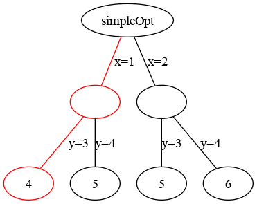
The tree for simpleOpt. The highlighted path represents one possible solution: x=1 and y=3.

The traveling salesman tree is a lot larger, but is straightforwards to construct.

The tree for exampleTsp. The highlighted path represents one possible solution: [0,1,2,..,12,13,14].

Note that the interior values associated with any particular choice are immaterial. All that matters is the structure of the edges. In the diagrams above, we notated each edge with the assignment it represents. The leaves are notated with solutions.

We can trivially encode such trees with a Haskell data type.

data Combinatorial a
   = Choice Int (Combinatorial a) [Combinatorial a]
   | Leaf a

Here, Choice represents a node with children. It contains one privileged child (the next in our path) along with a list of children not in our path. The Int argument is simply the cached degrees of freedom of the next child (more on this later). As expected Leaf is simply a node with no children, that represents the final result of a choice.

Combinatorial is trivially a Functor, and we can just ask GHC to figure that one out for us.

   deriving (Show, Functor)

Let’s define a function to figure out the number of degrees of freedom in a given Combinatorial. This helps in choosing a random neighbor.

Firstly, a single value has no degrees of freedom

degreesOfFreedom :: Combinatorial a -> Int
degreesOfFreedom Leaf {} = 0

A Choice has the degrees of freedom of its current child plus the possibilities of choosing one of its other subtrees.

degreesOfFreedom (Choice childSz _ remaining) = length remaining + childSz

We can also write a function to get the solution at the chosen path.

currentSolution :: Combinatorial a -> a
currentSolution (Leaf a) = a
currentSolution (Choice _ next _) = currentSolution next

A bit of thinking, and there are natural applicative and monadic interfaces ¹.

instance Applicative Combinatorial where
  pure = Leaf
  (<*>) = ap

instance Monad Combinatorial where
  return = pure
  Leaf a >>= b = b a
  Choice sz next rest >>= f =
    let next' = next >>= f
        sz'   = degreesOfFreedom next'
    in Choice sz' next' (map (>>= f) rest)

We can write a function to introduce non-determinism into Combinatorial. choose takes a non-empty list of possible values (the domain) of a variable; it yields the current choice. For the sake of simplicity, we error on an empty list, but a more robust solution would use Data.List.NonEmpty or another solution.

choose :: [a] -> Combinatorial a
choose [] = error "Empty domain"
choose [a] = Leaf a
choose (a:as) = Choice 0 (Leaf a) (map Leaf as)

Now, we can encode tsp in Combinatorial.

tspCombinatorial :: [ City ] -> (City -> City -> Double)
                 -> Combinatorial Double
tspCombinatorial [] _ = pure 0
tspCombinatorial (firstCity:cities) distance = go 0 firstCity cities
  where
    go curDistance lastCity [] = pure (distance firstCity lastCity + curDistance)
    go curDistance lastCity unvisited =
      do nextCity <- choose unvisited

         let unvisited' = filter (/=nextCity) unvisited
         go (curDistance + distance nextCity lastCity) nextCity unvisited'

For the problem above, we can form the set of all possible combinations.

exampleTsp :: Combinatorial Double
exampleTsp = tspCombinatorial allCities distFunc

Now, you may think that if we try to inspect exampleTsp, we’ll be in for a world of hurt. However, we can freely ask GHC for the value of tsp at the chosen path, without evaluating any other possible path. This is thanks to Haskell’s laziness – we can inspect partial solutions of the TSP problem without demanding the whole thing. Best of all, once we inspect the initial path, we never have to compute it again – the value of tsp at this path is cached, so long as we access it through exampleTsp.

*Main> currentSolution exampleTsp
817.0

Hitting the metal

So we now have a data structure in which to express a set of solutions along with a chosen solution and a strategy to search this set for a good enough solution. The only things we still need are one function to slightly perturb a solution and one to randomize it fully.

First, we’ll write a function to slightly perturb. We’ll consider a solution a slight perturbation of the current one if it chooses a different subtree at exactly one point in the current path. We’ll use degreesOfFreedom to figure out where to choose a different path. We’ll call these perturbations neighbors since they are “next” to the current solution.

We’ll use RandomGen from System.Random to abstract over our random generator.

pickNeighbor :: RandomGen g => Combinatorial a -> g -> (Combinatorial a, g)
pickNeighbor c g =
  let dof = degreesOfFreedom c
      (forkAt, g') = randomR (0, dof - 1) g
  in (neighborAt forkAt c, g')

neighborAt :: Int -> Combinatorial a -> Combinatorial a
neighborAt _ c@(Leaf {}) = c
neighborAt i (Choice sz next rest)
  | i < sz = let next' = neighborAt i next
             in Choice (degreesOfFreedom next') next' rest
  | otherwise =
      let restIdx = i - sz
          (restBefore, next':restAfter) = splitAt restIdx rest

          rest' = next:(restBefore ++ restAfter)
      in Choice (degreesOfFreedom next') next' rest'

Now, to randomize a given solution, we’ll just choose a random neighbor an arbitrary number of times.

randomize :: RandomGen g => Combinatorial a -> g -> (Combinatorial a, g)
randomize c g =
  let (numRandomizations, g') = randomR (0, degreesOfFreedom c) g

      randomizeNTimes 0 c g'' = (c, g'')
      randomizeNTimes n c g'' =
        let (c', g''') = pickNeighbor c g''
        in randomizeNTimes (n - 1) c' g'''
  in randomizeNTimes numRandomizations c g'

We are all set!

We can now define an anneal function that – given a Combinatorial and parameters for the annealing process – chooses a best guess. We’ll need to provide a random generator as well

type Temperature = Double
anneal :: ( RandomGen g )
       => ( energy -> energy -> Ordering)
       -> ( energy -> energy -> Temperature -> Double) -- ^ Probability of accepting a worse solution
       -> Temperature -- ^ Starting temperature
       -> Temperature -- ^ Ending temperature
       -> Double -- ^ Cooling factor
       -> Combinatorial energy -> g -> (Combinatorial energy, g)
anneal cmp acceptanceProbability tInitial tFinal coolingFactor initialSolution g =
  let (initial', g') = randomize initialSolution g

      doAnneal curTemp current best curRandom
        | curTemp <= tFinal = (best, curRandom)
        | otherwise =
            let (neighbor, curRandom') = pickNeighbor current curRandom

                currentValue = currentSolution current
                neighborValue = currentSolution neighbor

                (diceRoll, curRandom'') = randomR (0, 1) curRandom'
                acceptNeighbor = cmp neighborValue currentValue == LT ||
                                 acceptanceProbability currentValue neighborValue curTemp > diceRoll

                (current', current'Value) =
                  if acceptNeighbor
                  then (neighbor, neighborValue)
                  else (current, currentValue)

                best' = if cmp current'Value (currentSolution best) == LT
                        then current'
                        else best
            in doAnneal (curTemp * (1 - coolingFactor)) current' best' curRandom''
  in doAnneal tInitial initial' initial' g'

defaultAcceptanceProbability :: Double -> Double -> Temperature -> Double
defaultAcceptanceProbability curValue neighborValue curTemp =
  exp (-(neighborValue - curValue)/(curValue * curTemp))

Now we can solve our traveling salesman problem stochastically. First, a utility function to run the annealing in the IO monad using a new random generator.

runAnneal :: Temperature -> IO Double
runAnneal tInitial = do
  g <- newStdGen
  let (result, _) = anneal compare defaultAcceptanceProbability tInitial 1 0.003 exampleTsp g
  pure (currentSolution result)

Running it gives (results will obviously vary due to randomness):

*Main> runAnneal 100000
488.0

This is certainly better than the naïve solution of visiting every city in order:

*Main> head (tsp allCities distFunc)
817.0

Asking for directions

Because Combinatorial is a Monad, we can use all the normal Monad tricks. For example, if we want to get the path along with the length, we can use MonadWriter.

tspWithPath :: [ City ] -> (City -> City -> Double)
            -> WriterT [City] Combinatorial Double
tspWithPath [] _ = pure 0
tspWithPath (firstCity:cities) distance = go 0 firstCity cities
  where
    go curDistance lastCity [] = pure (distance firstCity lastCity + curDistance)
    go curDistance lastCity unvisited =
      do nextCity <- lift (choose unvisited)
         tell [nextCity]

         let unvisited' = filter (/=nextCity) unvisited
         go (curDistance + distance nextCity lastCity) nextCity unvisited'

exampleTspWithPath :: Combinatorial (Double, [City])
exampleTspWithPath = runWriterT (tspWithPath allCities distFunc)

runAnnealWithPath :: Temperature -> IO (Double, [City])
runAnnealWithPath tInitial = do
  g <- newStdGen
  let (result, _) = anneal (comparing fst) (defaultAcceptanceProbability `on` fst)
                           tInitial 1 0.003 exampleTspWithPath g
  pure (currentSolution result)

Of course, we can inspect the default solution without waiting for the universe to end

*Main> currentSolution exampleTspWithPath
(817.0,[1,2,3,4,5,6,7,8,9,10,11,12,13,14])

Running this we get

*Main> runAnnealWithPath 100000
(465.0,[10,5,3,12,1,2,6,8,4,7,9,11,13,14])

Discussion

In this article, we developed an intuition to express combinatorial optimization problems using monadic flattening. We then demonstrated two concrete monads which are of interest when solving optimization problems. We saw that choosing lists as our Combinatorial monad let us evaluate an optimization problem by examining every possible value of the objective function. We saw that our own custom Combinatorial monad allowed us to think of the set of solutions as a tree which can be searched through lazily. Finally, we used simulated annealing to search through the tree to achieve good enough optimizations of arbitrary problems.

Our annealing function is not limited to traveling salesman problems. We can encode any NP-complete problem where we can form an appropriate optimization metric. This is not just of theoretical significance. Database engines, for example, face the issue of join ordering for optimal query performance. Our little framework provides a way to describe these problems, and then to evaluate them fully when the search space is small or use an appropriate search method when they become intractable. This is similar to how RDBMSes like PostgreSQL optimize joins.

Because our tree structure comes with monadic operations, we don’t need to worry about coming up with specific representations of these problems, as libraries in other languages require. For example, the equivalent problem encoded in C using a standard simulated annealing library takes up almost 70 lines of code. In contrast, ours (the implementation of tsp) took only eleven, and could likely be simplified even more.

There are a few problems with our solution. First of all, we haven’t proven any kind of convergence to an optimal solution. Secondly, our data structure keeps around solutions which we’ve visited, but are known to be non-optimal. We could be smarter in allowing these solutions to be garbage collected and marked as inaccessible (a form of tabu search), or change our representation entirely to avoid this. It remains to be seen if this is useful.

Future work

Our tree-like structure for representing combinations can be thought of as containing the entire set of (as-yet uncomputed) solutions. In this article, we used simulated annealing to search through this structure for an optimal solution. However, there are multiple other strategies (termed meta-heuristics) we could use. It’s an interesting exercise for the reader to implement other search strategies, such as genetic algorithms, particle swarm optimization, or ant colony optimization. The possibilities are as endless as the possible paths through our fifteen cities!

Another interesting exploration would be to figure out what kinds of problems could be encoded using monads versus applicative. Above, we saw that the traveling salesman problem (which was NP-complete) requires the monadic bind. We expressed simpleOpt using monadic operations, but it could easily have been written using applicative. Part of me feels like there must be some interesting differences between those problems that need only applicatives, versus those that need monads.

These are thoughts for another day.