One question I have often been asked when it comes to Haskell is ‘how do I do dynamic programming?’.

For those of you unfamiliar, dynamic programming is an algorithmic technique where you solve a problem by building up some kind of intermediate data structure to reduce redundant work. This can sometimes turn exponential-time algorithms into polynomial-time ones.

One classical example of a problem requiring dynamic programming for manageable run-times is the longest common subsequence problem. This problem takes two inputs \(A\) and \(B\), and returns the length of the longest subsequence of elements in both \(A\) and \(B\). Recall that a subsequence \(L\) of a sequence \(S\) is a sequence of items \(\{s_{i_0},s_{i_1},\ldots,s_{i_n}\}\) where each \(s_{i_n} \in S\) and \(i_{m+1} > i_m\) for all \(m \in \{i_0, \ldots, i_n\}\). This differs from the longest common substring problem (a trivially polynomial algorithm) in that the items in \(L\) need not be contiguous in \(S\).

For example, the longest common subsequence of "babba" and "abca" is "aba", so our algorithm should return 3.

In an imperative programming language like C, a naïve programming solution might be ¹.

/* Returns length of LCS for X[0..m-1], Y[0..n-1] */
int lcs( char *X, char *Y, int m, int n )
{
   if (m == 0 || n == 0)
     return 0;
   if (X[m-1] == Y[n-1])
     return 1 + lcs(X, Y, m-1, n-1);
   else
     return max(lcs(X, Y, m, n-1), lcs(X, Y, m-1, n));
}

We can write a similar implementation in Haskell. Instead of iterating backwards, we’ll iterate forwards.

naiveLCS :: String -> String -> Int
naiveLCS [] _ = 0
naiveLCS _ [] = 0
naiveLCS (x:xs) (y:ys)
  | x == y    = 1 + naiveLCS xs ys
  | otherwise = max (naiveLCS (x:xs) ys) (naiveLCS xs (y:ys))

These implementations both have a runtime of \(O\left( n 2^m \right)\) given inputs of length \(m\) and \(n\).

This post is Literate Haskell. You can download this file and load it into GHCi without modification. If we evaluate naiveLCS with our first example, we get the answer fairly quickly:

*Main> naiveLCS "babba" "abca"
3

Let’s try to execute naiveLCS in GHCi with some larger inputs:

*Main> naiveLCS "nematode knowledge" "empty bottle"
7

Prepare to wait a while for the answer.

One way to speed things up is to note that we end up recursing on the same values over and over again. If we computed the results of the calls before they were needed, then we would not need to recompute them.

In C, this caching is straightforward. We just create an array to hold recursive steps we’ve already computed. If we ensure that our values are always computed before we need them, then we don’t even need to recurse ².

int lcs( char *X, char *Y, int m, int n )
{
   int L[m+1][n+1];
   int i, j;

   /* Following steps build L[m+1][n+1] in bottom up fashion. Note
      that L[i][j] contains length of LCS of X[0..i-1] and Y[0..j-1] */
   for (i=0; i<=m; i++)
   {
     for (j=0; j<=n; j++)
     {
       if (i == 0 || j == 0)
         L[i][j] = 0;

       else if (X[i-1] == Y[j-1])
         L[i][j] = L[i-1][j-1] + 1;

       else
         L[i][j] = max(L[i-1][j], L[i][j-1]);
     }
   }

   /* L[m][n] contains length of LCS for X[0..n-1] and Y[0..m-1] */
   return L[m][n];
}

The run-time of this algorithm is \(O\left(mn\right)\) where \(m\) and \(n\) are the sizes of the input strings.

This approach works well in imperative languages where in-place mutation is explicit. Of course, you can simulate the same kind of thing in Haskell with the IO or ST monad and the array package, but this seems inelegant. After all, the LCS function is a pure function – we ought to be able to craft a pure and efficient implementation.

It may seem like a major embarrassment that a functional language can’t implement this seemingly trivial function without exploding in computation time or demanding that we provide explicit, effectful instructions on how to mutate bits.

However, this conclusion is premature. Dynamic programming is no more difficult to implement in Haskell than in C. In fact, dynamic programming in Haskell seems trivially simple, because it takes the form of regular old Haskell recursion.

Mutation is everywhere

In Haskell, all functions are pure – their value is determined solely by their inputs. It is entirely possible to cache the values of Haskell functions to avoid recomputation. However, GHC and other popular Haskell compilers do not do this by default (see the MemoTrie package for a way to convince them to do so).

However, all Haskell compilers perform one particular kind of caching. If we have a variable binding of the form

let x = f a b c
in g x x x

then x is only computed once, each time it is used in g. This is due to Haskell’s laziness. Internally, the expression g x x x results in an unevaluated thunk, where each instance of x points to the same unevaluated thunk f a b c. When x is demanded once in g, the thunk is computed, and future evaluations of the thunk pointed to by x simply use the cached value. This is demonstrated in the figure below.

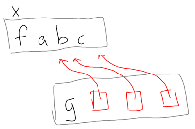
The heap layout of the expression let x = f a b c in g x x x. Notice how each occurrence of x in the invocation of g points to the same thunk for f.

This feature is called ‘sharing’. You may think this sounds suspiciously like mutation in a pure language, and you’d be absolutely right. Contrary to popular belief, mutation is prevalent during the execution of any Haskell program. In fact, it’s integral to the language. The difference is that mutation is controlled, and while a mutation may change the value in a certain memory cell, it never changes its semantics. This is known as referential transparency.

We can use this technique to cache values. A common example of this is the one-line Fibonacci many Haskell beginners encounter. Firstly, the naive Fibonacci function. This has complexity \(O(\phi^n)\), where \(\phi\) is the golden ratio.

naiveFib :: Int -> Int
naiveFib 0 = 0
naiveFib 1 = 1
naiveFib n = naiveFib (n - 1) * naiveFib (n - 2)

The one-line solution uses a lazy list to represent all Fibonacci numbers, and then list lookups to compute the \(n^{\text{th}}\) number.

linearFib :: Int -> Int
linearFib n = let fibs = 0:1:zipWith (+) fibs (tail fibs)
              in fibs !! n

Note that, aside from the first two entries, each entry depends on the values of the entry computed within the list, as illustrated below.

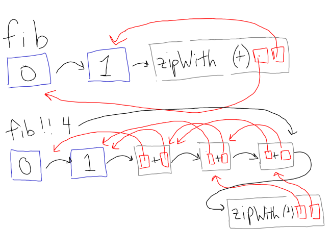
Dependencies for the fibonnaci ‘one-liner’. When we evaluate fibs !! 4, we get a reference to a thunk that depends on other thunks in the fibs list. This causes each thunk to only be computed once.

When we compute fibs !! 4, we get a reference for a thunk that has yet to be computed. When we force the value, each referenced cell is computed, but never more than once. Thus, the time complexity of linearFib is simply O(n).

Finding subsequences

We can apply the exact same optimization to the longest-common-subequence as the Fibonacci problem. The data flow is a bit harder to visualize, because the LCS problem uses a ‘two-dimensional’ data structure to hold unevaluated thunks.

In this case, we’re going to go with the most obvious solution. This solution isn’t going to be as fast as an optimized one, but it will have the correct \(O(mn)\) complexity.

First, let’s write our function signature and a simple case if one of the strings is empty.

dpLCS :: String -> String -> Int
dpLCS _ [] = 0
dpLCS a b =

Looking at the C solution, we can demonstrate how each entry in the array depends on others. Note that each entry depends only on the entries to the left, directly above, and diagonal top-left, as illustrated in the diagram below. Notice also how each column corresponds to a specific index into the second string, and each row to a specific index in the first.

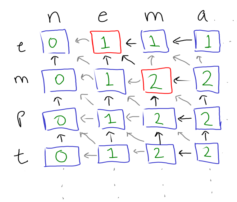
The table built up by the imperative algorithm for the inputs “nematode knowledge” and “empty bottle”. The arrows point to cells that were necessary to compute the cell they originate from. Dark arrows represent dependencies actually used to compute this cell. Red boxes are cells where we added one because the corresponding characters matched.

With that in mind, we can construct a function to construct a row in this table, given the row directly above and the character in the first string being considered.

  let nextRow ac prevRow =

To keep the computation of each entry orthogonal, notice that we can think of the entries on the left and upper edges as being computed the same as every other entry, except with zeros in the diagonal and left or upper entries respectively. These ‘phantom’ nodes are illustrated below.

With that in mind, we can construct a list of elements on the diagonal. The diagonal entry used to calculate the first element is simply zero. For the second element, it’s the first element in the row above; for the third, the second; etc.

         let diagonals = 0:prevRow

We can also construct a list for elements to the left. The element to the left of the first is simply zero. The element to the left of the second is the first, etc.

             lefts = 0:thisRow

Above, thisRow corresponds to the final value of this row, which has yet to be computed. This is where the caching magic takes place.

Finally, the elements directly above is simply the previous row.

             ups = prevRow

Now, we only care about the max of the solution to the left and the solution above, so we can construct a list of maxes we care about.

             maxes = zipWith max lefts ups

Now, we can compute this row, by simply combining these maxes with the diagonal values and the character corresponding to the column.

             thisRow = zipWith3 (\diag maxLeftUp bc ->
                                   if bc == ac then 1 + diag else maxLeftUp)
                                   diagonals maxes b

Finally, we need to return the value of thisRow.

        in thisRow

Now, we can construct our entire table, keeping in mind that the ‘previous row’ corresponding to the first row, is simply the row containing all zeros.

      firstRow = map (\_ -> 0) b
      dpTable = firstRow:zipWith nextRow a dpTable

Now, the actual value we’re interested in is simply the very last element of the very last list. We can just use Haskell’s last function to get this value. Because of our initial check, this usage is safe.

  in last (last dpTable)

Now, if we run dpLCS on our little problem, we get the answer instantaneously.

*Main> dpLCS "nematode knowledge" "empty bottle"
7

For clarity’s sake, the complete implementation of dpLCS is given below:

dpLCS :: String -> String -> Int
dpLCS _ [] = 0
dpLCS a b =
  let nextRow ac prevRow =
        let diagonals = 0:prevRow
            lefts = 0:thisRow
            ups = prevRow
            maxes = zipWith max lefts ups
            thisRow = zipWith3 (\diag maxLeftUp bc ->
                                   if bc == ac then 1 + diag else maxLeftUp)
                                   diagonals maxes b
        in thisRow

      firstRow = map (\_ -> 0) b
      dpTable = firstRow:zipWith nextRow a dpTable

  in last (last dpTable)

Discussion

The solution above has the right complexity, but is quite inefficient. While it exploits laziness to avoid recomputation, it is too lazy in some respects. In a future post, we’ll see how to control Haskell’s sharing to get performance we need. We’ll also see that Haskell’s approach to these problems gives us some important memory properties for free.